Mineral Potential Mapping using Geochemistry Data
Exploration of Statistical Methods to Assess Stream Sediment and Soil Sampling Results
Latar Belakang
Proyek ini merupakan soal UAS Geokimia Eksplorasi, di mana diberikan 2 dataset: [Soil Sample Data, Stream Sediment Data]. Perlu diketahui bahwa dalam eksplorasi Cu-Au, Stream Sediment Sampling (SSS) dilakukan terlebih dahulu, baru kemudian Soil Sampling (SS) akan dilakukan pada area yang lebih berpotensi yang diketahui dari SSS. Ujian ini memberikan 2 tugas utama: Lakukan klasterisasi data (minimal 3 klaster), Buat Peta Anomali Tiap unsur.
Metode
Klasterisasi akan menggunakan pendekatan principal component analysis (PCA) dan k-means clustering (KMC) sedangkan peta anomali akan menggunakan aplikasi surfer untuk menginterpolasi data.
Output
1. Klasterisasi
A. Deskripsi Data
1
2
3
4
5
6
7
8
9
10
# import library
import numpy as np
import scipy as sc
import matplotlib.pyplot as plt
import pandas as pd
import seaborn as sns

# import dataset
soil = pd.read_csv("soil.csv", delimiter=',')
stream = pd.read_csv("stream.csv", delimiter=';')
1
2
# deskripsi data stream sediment sampling
print(stream.describe())
1
2
3
4
5
6
7
8
9
10
11
12
13
14
15
16
17
18
19
           Northing        Easting    Elevation          Au          Ag  \
count  1.130000e+02     113.000000   113.000000  113.000000  113.000000
mean   9.795687e+06  749714.548673  1229.380531    0.004376    0.069027
std    1.023627e+03     839.607572    40.986348    0.003059    0.042426
min    9.794083e+06  748207.000000  1146.000000    0.002500    0.050000
25%    9.794859e+06  749068.000000  1199.000000    0.002500    0.050000
50%    9.795451e+06  749692.000000  1224.000000    0.002500    0.050000
75%    9.796515e+06  750225.000000  1257.000000    0.006000    0.100000
max    9.798096e+06  751401.000000  1346.000000    0.017000    0.400000

               As          Cu          Mo          Pb          Sb          Zn
count  113.000000  113.000000  113.000000  113.000000  113.000000  113.000000
mean     6.353982   29.716814    1.340708   15.176991    0.929204   62.991150
std      5.990946   19.983238    1.498907   11.950217    0.485813   36.442346
min      1.000000    7.000000    0.500000    4.000000    0.500000   27.000000
25%      3.000000   21.000000    0.500000   10.000000    0.500000   46.000000
50%      4.000000   26.000000    1.000000   13.000000    1.000000   58.000000
75%      8.000000   33.000000    1.000000   18.000000    1.000000   73.000000
max     32.000000  146.000000   10.000000  109.000000    3.000000  383.000000
1
2
# deskripsi data soil sampling
print(soil.describe())
1
2
3
4
5
6
7
8
9
10
11
12
13
14
15
16
17
18
19
20
21
22
23
24
25
26
27
28
29
           Northing        Easting    Elevation       Depth          Au  \
count  2.420000e+02     242.000000   242.000000  242.000000  242.000000
mean   9.795762e+06  749275.483471  1294.037190   84.359504    0.012308
std    1.041078e+02     274.960642    31.628462   13.173865    0.035687
min    9.795471e+06  748698.000000  1231.000000   50.000000    0.002500
25%    9.795710e+06  749056.500000  1264.000000   80.000000    0.002500
50%    9.795777e+06  749285.000000  1303.500000   85.000000    0.006000
75%    9.795826e+06  749530.500000  1321.000000   90.000000    0.008750
max    9.795991e+06  749737.000000  1345.000000  140.000000    0.460000

               Ag          As          Cu          Mo          Pb          Sb  \
count  242.000000  242.000000  242.000000  242.000000  242.000000  242.000000
mean     0.243182   17.847107   27.355372    0.900826   14.231405    1.324380
std      0.131875   30.253105   13.115421    0.415568    5.971246    4.169035
min      0.050000    1.000000    2.000000    0.500000    3.000000    0.500000
25%      0.100000    5.000000   20.000000    0.500000   10.000000    0.500000
50%      0.300000    7.000000   29.000000    1.000000   13.000000    0.500000
75%      0.300000   14.000000   34.000000    1.000000   16.750000    0.500000
max      0.700000  244.000000  114.000000    4.000000   52.000000   49.000000

               Zn
count  242.000000
mean    65.305785
std     23.104074
min      4.000000
25%     52.000000
50%     71.000000
75%     81.000000
max    118.000000
1
2
3
4
# Sebaran spasial data SSS
sns.scatterplot(x = stream['Easting'], y = stream['Northing']).set(title='Sebaran data Stream Sediment Sample')
plt.show()
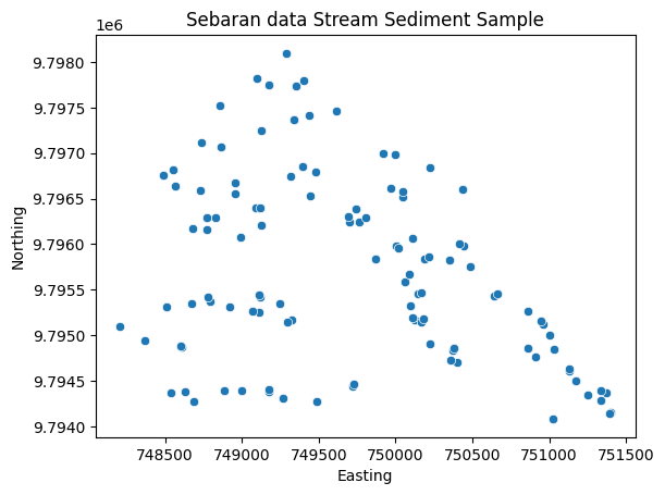 Sebaran data Stream Sediment Sampling.
1
2
3
# Sebaran spasial data SS
sns.scatterplot(x = soil['Easting'], y = soil['Northing']).set(title='Sebaran data Soil Sampling')
plt.show()
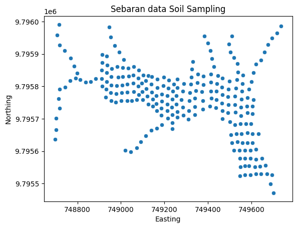 Sebaran data Soil Sampling.
1
2
3
4
# ambil parameter koordinat
coordinates = ["Northing", "Easting"]
costream = stream[coordinates]
cosoil = soil[coordinates]
1
2
3
4
5
6
# korelasi antar unsur SSS
streamm = ["Au", "Ag", "As", "Cu", "Mo", "Pb", "Sb", "Zn"]
streamn = stream[streamm]

heatmap = sns.heatmap(streamn.corr(), cmap="YlGnBu", annot=True)
plt.show()
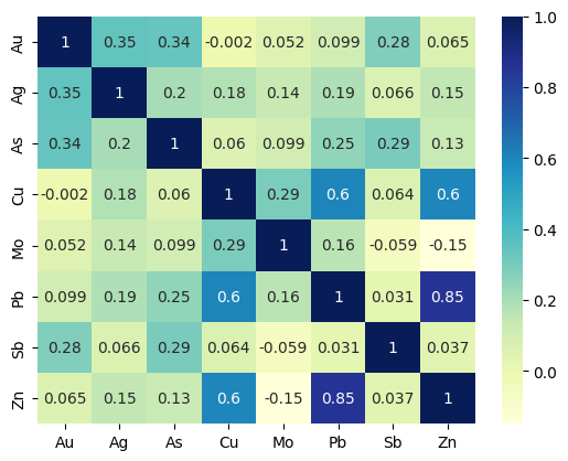 Heatmap Stream Sediment Sampling.
1
2
3
4
5
6
# korelasi antar unsur SS
soilm = ["Au", "Ag", "As", "Cu", "Mo", "Pb", "Sb", "Zn"]
soiln = soil[soilm]

heatmap = sns.heatmap(soiln.corr(), cmap="YlGnBu", annot=True)
plt.show()
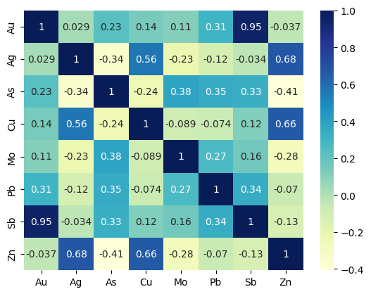 Heatmap Soil Sampling.
B. Principal Component Analysis
Pada proses ini, akan dilakukan reduksi dimensi, sehingga hanya terdapat beberapa parameter yang memiliki explained variance >70%. Dalam hal ini, data SSS membutuhkan 4 principal component (PC), sedangkan data SS membutuhkan 3 PC saja.
1
2
3
4
5
6
7
8
9
10
11
12
13
14
15
16
17
18
19
20
21
22
23
24
25
26
27
28
29
30
31
32
33
34
from sklearn.preprocessing import RobustScaler
from sklearn.preprocessing import PowerTransformer
from sklearn.preprocessing import QuantileTransformer
from sklearn.preprocessing import StandardScaler
from sklearn.decomposition import PCA

# Stream Sediment Sampling
# Standarisasi
sss = StandardScaler().fit_transform(streamn)
# fitting
pcasss = PCA(n_components=8)
componentsss = pcasss.fit_transform(sss)
PC_valuesss = np.arange(pcasss.n_components_) + 1
plt.plot(PC_valuesss,
        pcasss.explained_variance_ratio_,
        'o-',
        linewidth=2,
        color='blue')
plt.title('Scree Plot Stream Sediment Sampling')
plt.xticks([1, 2, 3, 4, 5, 6, 7, 8])
plt.xlabel('Principal Component')
plt.ylabel('Variance Explained')
plt.show()
# PCA Components
print("PCA Komponen: \n", abs(pcasss.components_))
explained_variance = pcasss.explained_variance_ratio_
print("explained variance: \n", explained_variance)
loadingsss = pcasss.components_.T * np.sqrt(pcasss.explained_variance_)
print("loadings: \n", loadingsss)

# mengambil 3 komponen saja
pcas = PCA(n_components=3)
componentsss = pcas.fit_transform(sss)
data_pca_sss = pd.DataFrame(data=componentsss, columns=['PC1', 'PC2', 'PC3'])
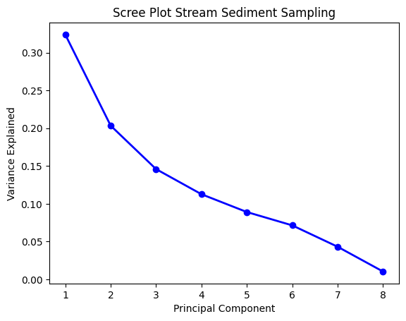 Screeplot PC Stream Sediment Sampling.
1
2
3
4
5
6
7
8
9
10
11
12
13
14
15
16
17
18
19
20
21
22
23
24
25
26
27
28
29
30
31
32
33
34
35
36
37
PCA Komponen:
 [[0.19187024 0.25994356 0.25220231 0.472332   0.1332234  0.5540761
  0.12770889 0.51754543]
 [0.56300724 0.31584221 0.45953616 0.24962305 0.04131893 0.20264922
  0.44275346 0.26641472]
 [0.00956807 0.27145768 0.06124515 0.17747241 0.82339094 0.06851128
  0.32117508 0.32427131]
 [0.26388953 0.64159068 0.25996068 0.17254489 0.35499856 0.025459
  0.53082358 0.11369527]
 [0.03795414 0.2514599  0.69461527 0.31345984 0.00985173 0.1748355
  0.56784124 0.03836362]
 [0.74734345 0.5247963  0.32561651 0.01394463 0.12862289 0.08915249
  0.17360899 0.07220768]
 [0.12712045 0.09315561 0.24927682 0.73231464 0.29891363 0.4569437
  0.22384632 0.16877401]
 [0.01889618 0.00489485 0.05687332 0.13633179 0.26562641 0.63188436
  0.00646296 0.71268579]]
explained variance:
 [0.32406392 0.20344352 0.14592823 0.11265931 0.08907845 0.0714307
 0.04310626 0.01028961]
loadings:
 [[ 0.31031171 -0.72145811 -0.01038411  0.25164071 -0.03218257 -0.56746345
   0.07498265  0.00544564]
 [ 0.42040669 -0.40473179  0.29460966  0.61181031 -0.21322115  0.39848174
  -0.05494832  0.00141063]
 [ 0.40788675 -0.58886648 -0.0664686  -0.24789422  0.5889872   0.24724304
   0.14703722 -0.01639016]
 [ 0.76390247  0.31987612  0.19260861 -0.16453597 -0.26579294  0.01058826
   0.43195956  0.03928907]
 [ 0.21546218 -0.05294759  0.89361602 -0.33852078  0.00835361 -0.09766432
  -0.17631574 -0.07655011]
 [ 0.89610719  0.25968213 -0.07435445 -0.02427728  0.14824879 -0.06769415
  -0.2695306   0.18210094]
 [ 0.20654356 -0.56736051 -0.34856735 -0.50618462 -0.48149132  0.1318226
  -0.13203691 -0.00186254]
 [ 0.83702615  0.34139359 -0.35192765  0.10841794  0.03252978 -0.05482783
  -0.09955222 -0.20538687]]
1
2
3
4
5
6
7
8
9
10
11
12
13
14
15
16
17
18
19
20
21
22
23
24
25
26
27
28
# Stream Sediment Sampling
# Standarisasi
ss = StandardScaler().fit_transform(soiln)
# fitting tes
pcass = PCA(n_components=8)
componentss = pcass.fit_transform(ss)
PC_valuess = np.arange(pcass.n_components_) + 1
plt.plot(PC_valuess,
        pcass.explained_variance_ratio_,
        'o-',
        linewidth=2,
        color='blue')
plt.title('Scree Plot Soil Sampling')
plt.xticks([1, 2, 3, 4, 5, 6, 7, 8])
plt.xlabel('Principal Component')
plt.ylabel('Variance Explained')
plt.show()
# PCA Components
print("PCA Komponen: \n", abs(pcass.components_))
explained_variance = pcass.explained_variance_ratio_
print("explained variance: \n", explained_variance)
loadingss = pcass.components_.T * np.sqrt(pcass.explained_variance_)
print("loadings: \n", loadingss)

# mengambil 3 komponen saja
pc = PCA(n_components=3)
componentss = pc.fit_transform(ss)
data_pca_ss = pd.DataFrame(data=componentss, columns=['PC1', 'PC2', 'PC3'])
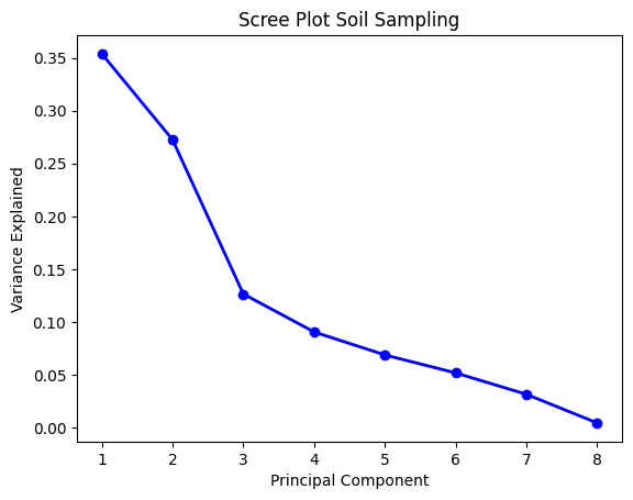 Screeplot PC Soil Sampling.
1
2
3
4
5
6
7
8
9
10
11
12
13
14
15
16
17
18
19
20
21
22
23
24
25
26
27
28
29
30
31
32
33
34
35
36
37
PCA Komponen:
 [[0.25717541 0.40782702 0.42716077 0.33200723 0.30768537 0.28362766
  0.30967742 0.45147288]
 [0.54750278 0.32132918 0.05043709 0.40949871 0.02680319 0.24001289
  0.5279991  0.29941197]
 [0.34377274 0.16093001 0.27196637 0.24301009 0.64432738 0.40730594
  0.30165204 0.22550472]
 [0.09265709 0.00498547 0.04540232 0.25393928 0.53050676 0.78047057
  0.11132689 0.1479117 ]
 [0.12641922 0.14527307 0.85096514 0.12075254 0.41069418 0.22270364
  0.04541753 0.06214266]
 [0.06567812 0.76093541 0.02986977 0.61669095 0.14820255 0.06481802
  0.01970675 0.09439298]
 [0.16079029 0.32301269 0.10127755 0.44556875 0.1316913  0.18094617
  0.00192298 0.78162192]
 [0.67910789 0.00609871 0.06059449 0.07157191 0.00630966 0.01941447
  0.72074574 0.10044847]]
explained variance:
 [0.35372096 0.27247903 0.12651242 0.09061089 0.06881786 0.05182689
 0.03156874 0.00446321]
loadings:
 [[ 0.43351486  0.81002239  0.34656298 -0.07905203 -0.09399567 -0.04237819
  -0.08097157 -0.12858986]
 [-0.68746494  0.47540184 -0.1622362  -0.00425344  0.10801395 -0.49098647
   0.16266434 -0.0011548 ]
 [ 0.7200554   0.07462094 -0.27417378 -0.03873579  0.63271264 -0.01927319
  -0.05100186 -0.01147364]
 [-0.5596572   0.60584738 -0.24498248 -0.21665276  0.08978236  0.39791408
   0.22438173 -0.01355222]
 [ 0.51865838  0.03965493 -0.64955707 -0.45261118 -0.3053608  -0.09562631
  -0.06631776  0.00119474]
 [ 0.47810483  0.35509558 -0.41061184  0.6658722  -0.1655854   0.04182322
   0.09112178 -0.00367615]
 [ 0.52201633  0.78116698  0.3041004  -0.0949805  -0.033769   -0.0127156
   0.00096838  0.13647404]
 [-0.76103779  0.44297565 -0.22733504  0.12619347  0.04620453  0.06090619
  -0.39361306  0.01902003]]
C. K-Means Clustering
Data akan dibagi menjadi beberapa klaster (minimal 3) menggunakan algoritma KMC
Berdasarkan nilai silhouette score terbesar, data SSS memiliki jumlah klaster ideal 4, sedangkan data SS sejumlah 5.
1. Memeriksa Jumlah Klaster ideal
1
2
3
4
5
6
7
8
9
10
11
12
13
14
15
16
17
18
19
20
21
22
23
24
25
26
27
28
29
30
31
32
33
34
35
36
37
38
39
40
from sklearn.cluster import KMeans
from sklearn.metrics import silhouette_score
from sklearn.pipeline import Pipeline

def silKMC(df, nama):
    x = df.iloc[:, 0:8].values
    sc = []
    K = range(3, 20)
    for k in K:
        # Building and fitting the model
        # membuat pipeline untuk preprocessor
        preprocessor = Pipeline([("scaler", RobustScaler()),
                                 ("pca", PCA(n_components=3,
                                             random_state=None))])
        # membuat pipeline untuk clusterer
        clusterer = Pipeline([("KMC",
                               KMeans(n_clusters=k,
                                      init="k-means++",
                                      n_init=50,
                                      max_iter=500,
                                      random_state=42))])
        # membuat pipeline untuk fitting
        pipe = Pipeline([("preprocessor", preprocessor),
                         ("clusterer", clusterer)])
        # Data Lengkap
        pipe.fit_predict(x)
        pra = pipe["preprocessor"].transform(x)
        pasca = pipe.fit_predict(x)
        score = silhouette_score(pra, pasca, metric="euclidean")
        sc.append(score)
    figx, ax = plt.subplots()
    plt.plot(K, sc)
    plt.xticks(np.arange(3, 21, 1.0))
    plt.xlabel('Jumlah Klaster')
    plt.ylabel('Silhouette Score')
    plt.title(f"Silhouette Score K-Means Clustering {nama}")
    plt.show()

silKMC(streamn, "Stream Sediment Sampling")
silKMC(soiln, "Soil Sampling")
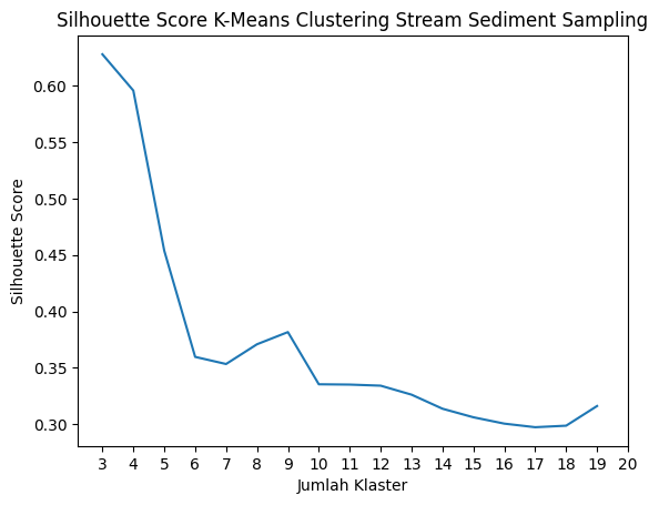 Screeplot Silhouette Score Stream Sediment Sampling.
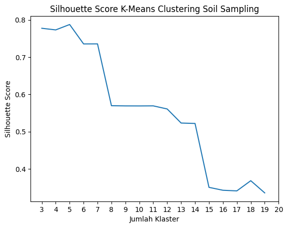 Screeplot Silhouette Score Soil Sampling.
2. K-Means Clustering
1
2
3
4
5
6
7
8
9
10
11
12
13
14
15
16
17
18
19
20
21
22
23
24
25
26
27
28
29
30
31
32
33
34
35
36
37
38
39
40
41
42
43
44
45
46
47
48
49
50
51
52
53
54
55
56
57
58
59
60
61
62
63
64
65
66
67
68
69
70
71
72
73
74
75
76
77
78
79
80
81
82
83
84
85
86
87
88
89
90
91
92
93
94
95
96
97
98
99
100
101
102
103
104
105
106
107
108
109
110
111
112
113
114
115
116
117
118
119
120
121
122
123
124
125
126
def kmc(nama, df, parameter, loadings, data_pca, jumlah_klaster, coor):
x = df.iloc[:, 0:8].values
# Membuat pipeline untuk preprocessor
preprocessor = Pipeline([("scaler", RobustScaler()),
("pca", PCA(n_components=3, random_state=None))])
# Membuat pipeline untuk clusterer
clusterer = Pipeline([("kmeans",
KMeans(n_clusters=jumlah_klaster,
init="k-means++",
n_init=50,
max_iter=500,
random_state=42))])
# Membuat pipeline untuk fitting
pipe = Pipeline([("preprocessor", preprocessor), ("clusterer", clusterer)])
# Melukukan prediksi terhadap Dataset
pipe.fit(x)
pipe.predict(x)
pra = pipe["preprocessor"].transform(x)
pasca = pipe["clusterer"]["kmeans"].labels_
# silhouette_score
score = silhouette_score(pra, pasca, metric="euclidean")
print(f'silhouette score KMC: {score}')
# Tambah data pada datafrane PCA
pcadf = data_pca
pcadf["predicted_cluster"] = pasca
pcadf["Latitude"] = coor["Northing"]
pcadf["Longitude"] = coor["Easting"]
pcadf.to_csv(f"csv {nama}.csv")
# Plot dataset
fig, ax = plt.subplots(figsize=(15, 10))
sns.scatterplot(x="PC1",
y="PC2",
edgecolors="black",
linewidth=0.5,
s=300,
data=pcadf,
hue="predicted_cluster",
palette="plasma")
plt.legend(fontsize="large", loc=1)
ax.axhline(y=0, color='gray', alpha=0.5)
ax.axvline(x=0, color='gray', alpha=0.5)
for i, feature in enumerate(parameter):
plt.arrow(0,
0,
4 * loadings[i, 0],
4 * loadings[i, 1],
color='black',
width=0.01,
head_width=0.1)
plt.text(4.2 * loadings[i, 0],
4.2 * loadings[i, 1],
feature,
color = "red",
fontsize="large")
plt.title(f"{nama}")
plt.show()
fig2, ax = plt.subplots(figsize=(15, 10))
sns.scatterplot(x="PC1",
y="PC3",
edgecolors="black",
linewidth=0.5,
s=300,
data=pcadf,
hue="predicted_cluster",
palette="plasma")
plt.legend(fontsize="large", loc=1)
ax.axhline(y=0, color='gray', alpha=0.5)
ax.axvline(x=0, color='gray', alpha=0.5)
for i, feature in enumerate(parameter):
plt.arrow(0,
0,
4 * loadings[i, 0],
4 * loadings[i, 1],
color='black',
width=0.01,
head_width=0.1)
plt.text(4.2 * loadings[i, 0],
4.2 * loadings[i, 1],
feature,
color = "red",
fontsize="large")
plt.title(f"{nama}")
plt.show()
fig3, ax = plt.subplots(figsize=(15, 10))
sns.scatterplot(x="PC2",
y="PC3",
edgecolors="black",
linewidth=0.5,
s=300,
data=pcadf,
hue="predicted_cluster",
palette="plasma")
plt.legend(fontsize="large", loc=1)
ax.axhline(y=0, color='gray', alpha=0.5)
ax.axvline(x=0, color='gray', alpha=0.5)
for i, feature in enumerate(parameter):
plt.arrow(0,
0,
4 * loadings[i, 0],
4 * loadings[i, 1],
color='black',
width=0.01,
head_width=0.1)
plt.text(4.2 * loadings[i, 0],
4.2 * loadings[i, 1],
feature,
color = "red",
fontsize="large")
plt.title(f"{nama}")
plt.show()
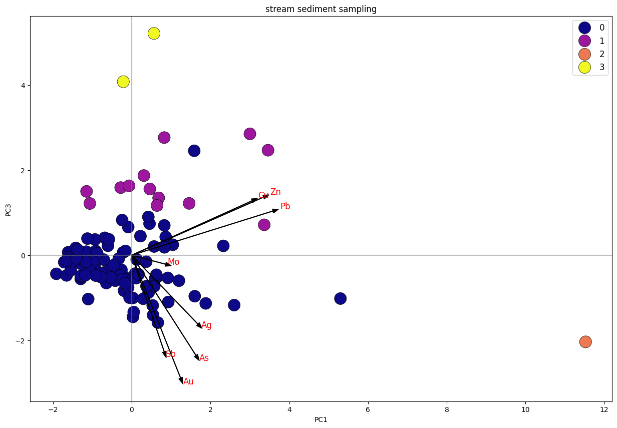
kmc("stream sediment sampling", streamn, streamm, loadingsss, data_pca_sss, 4, costream)
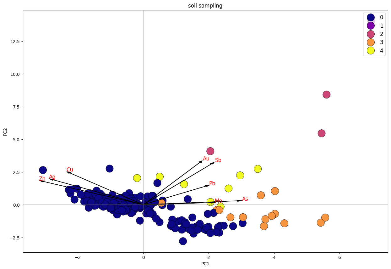
kmc("soil sampling", soiln, soilm, loadingss, data_pca_ss, 5, cosoil)
1
silhouette score KMC: 0.5955732674747102
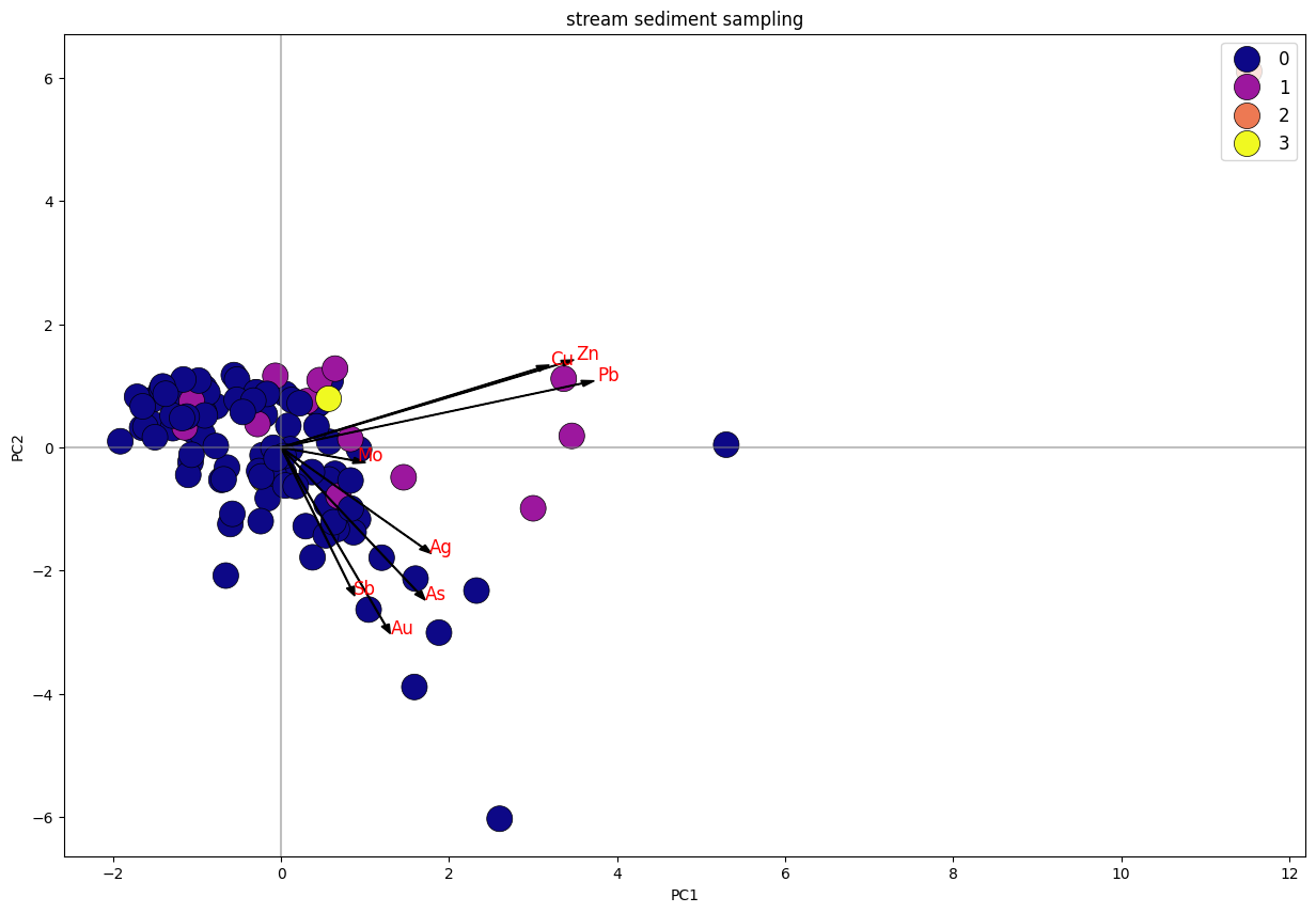 Biplot K-Means Clustering PC1 Vs. PC2 Stream Sediment Sampling.
 Biplot K-Means Clustering PC1 Vs. PC3 Stream Sediment Sampling.
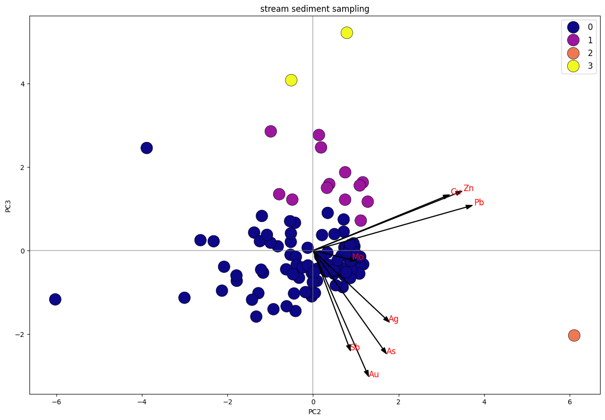 _Biplot K-Means Clustering PC2 Vs. PC3
1
silhouette score KMC: 0.7876141221589223
 Biplot K-Means Clustering PC1 Vs. PC2 Stream Sediment Sampling.
 Biplot K-Means Clustering PC1 Vs. PC3 Stream Sediment Sampling.
 Biplot K-Means Clustering PC2 Vs. PC3
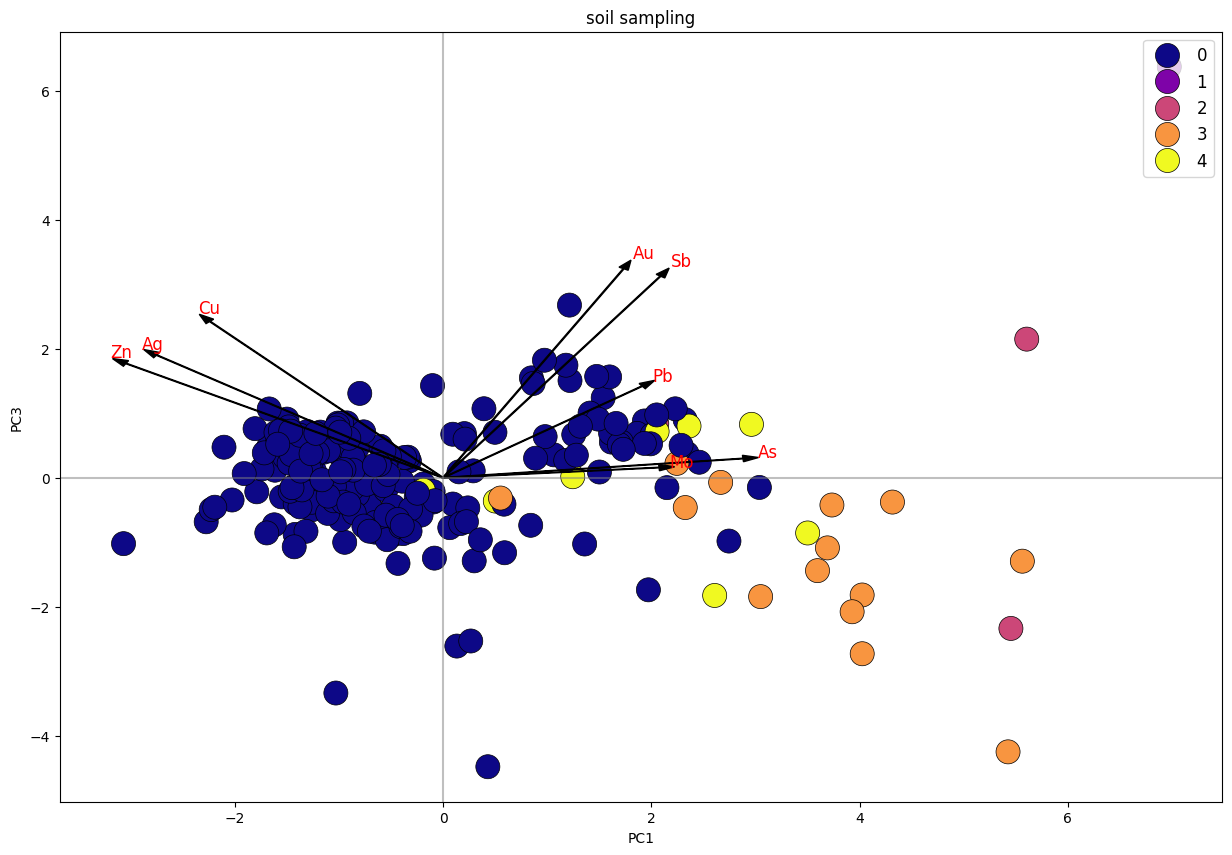
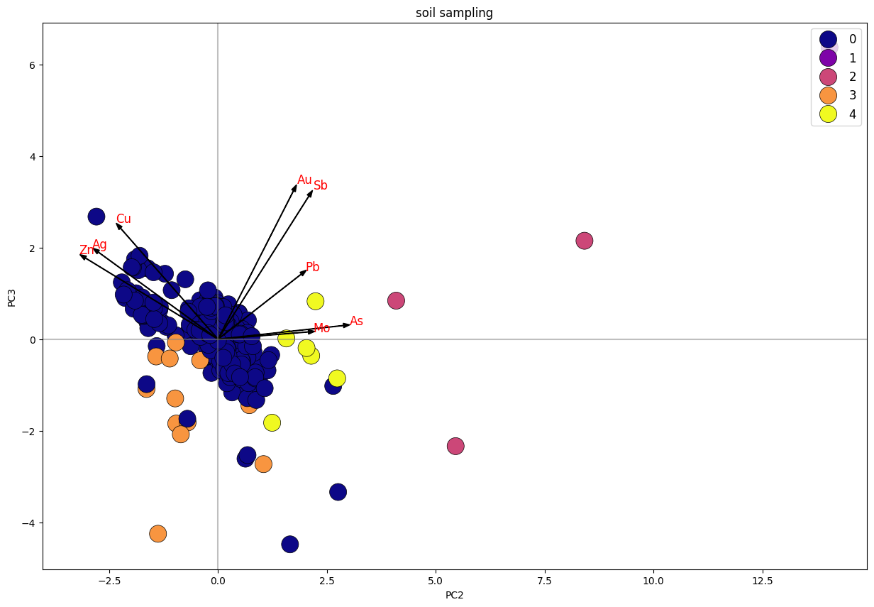
Dari plot stream sediment sampling, dapat diketahui bahwa data terbagi menjadi 4 klaster, di mana klaster 1 dan 3 memiliki trend searah dengan unsur Cu, Pb, Zn. sedangkan klaster 1 tersebar merata mengikuti trend unsur Cu-Pb-Zn dan trend Au-As-Ag-Sb. Klaster 2 merupakan anomali.
Pada plot soil sampling, dapat diketahui klaster 0 memiliki 2 arah trend, yakni yang positif dengan unsur Cu-Ag-Zn dan Au-Sb-Pb. sedangkan klaster lainnya positif dengan unsur Au-Sb-Pb.
2. Peta Anomali
A. Peta Anomali Data Stream Sediment Sampling
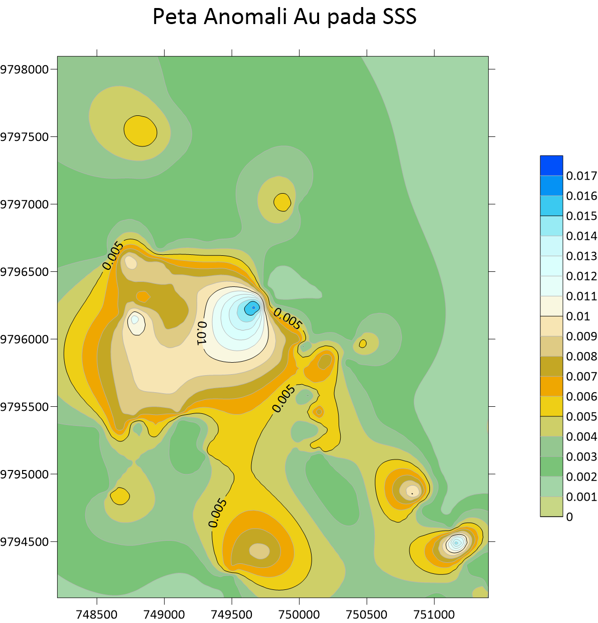 Peta Anomali Au Stream Sedimen
 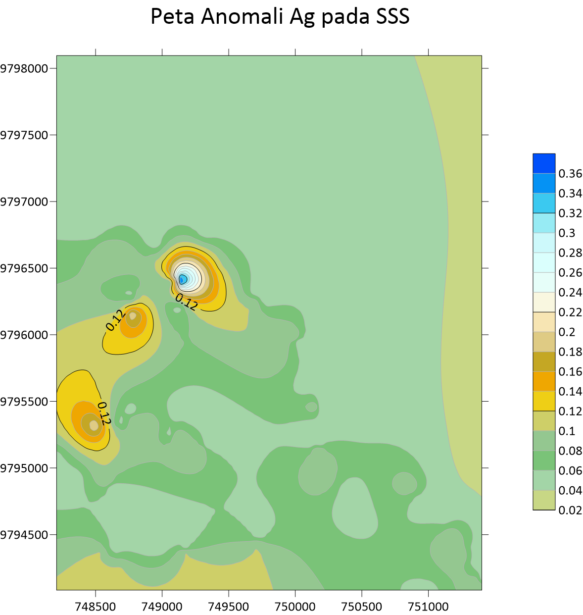 Peta Anomali Ag Stream Sedimen Sampling
 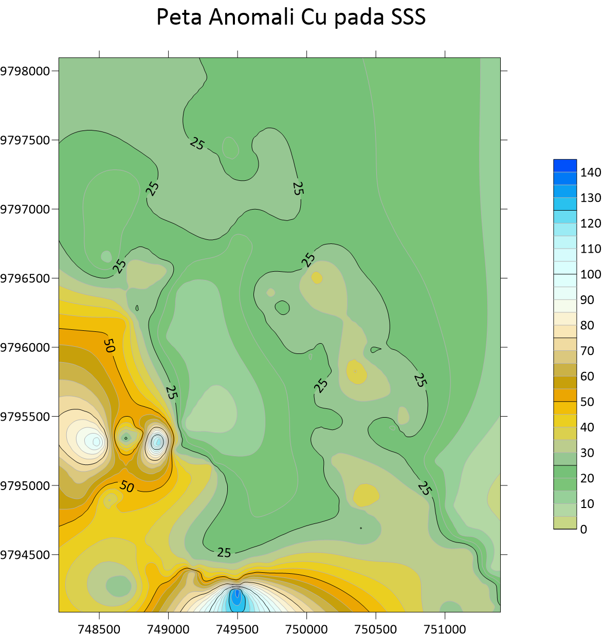 Peta Anomali Cu Stream Sedimen Sampling
 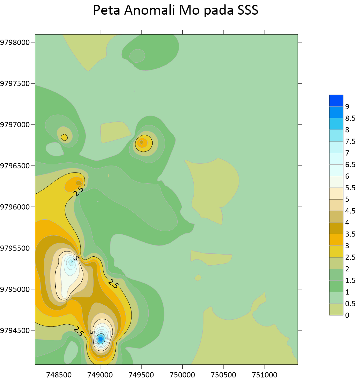 Peta Anomali Mo Stream Sedimen Sampling
 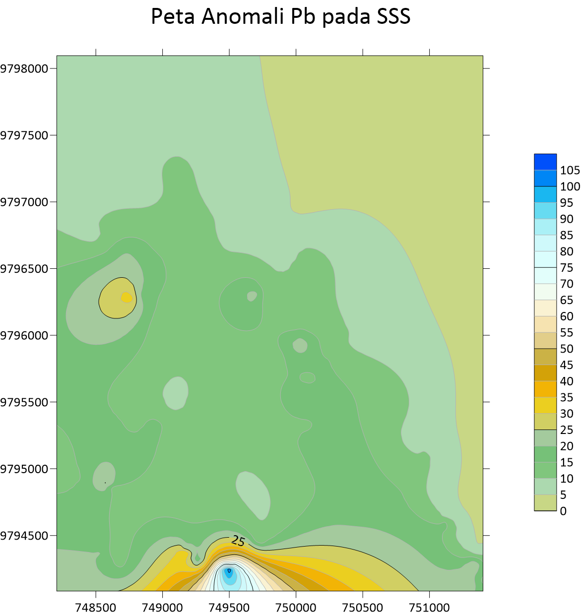 Peta Anomali Pb Stream Sedimen Sampling
 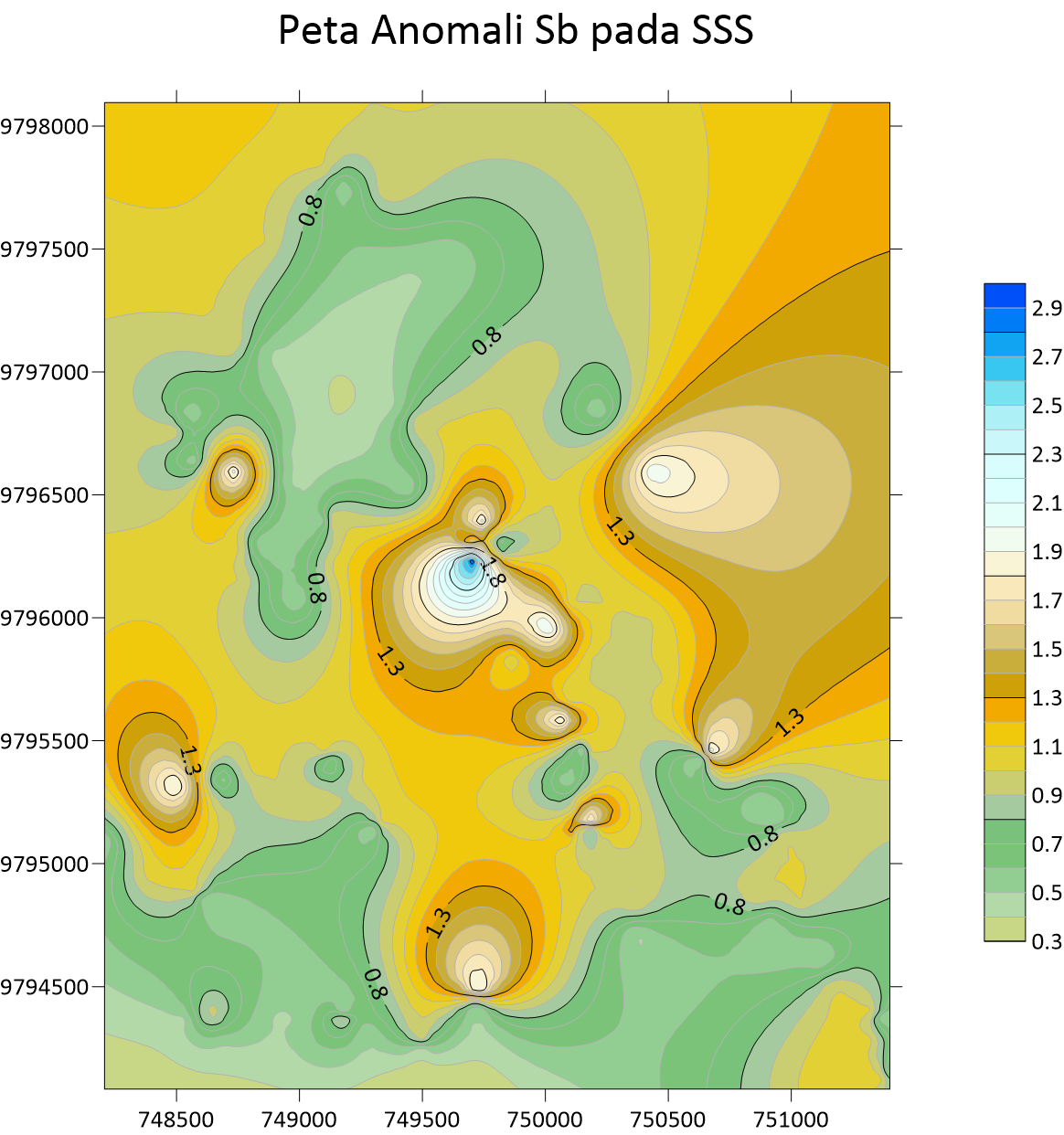 Peta Anomali Sb Stream Sedimen Sampling
 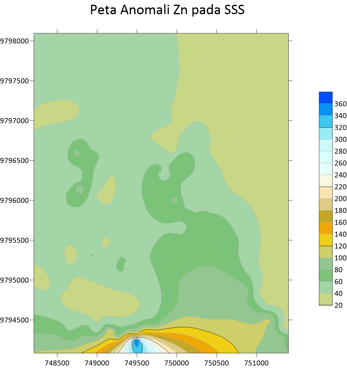 Peta Anomali Zn Stream Sedimen Sampling
B. Peta Anomali Data Soil Sampling
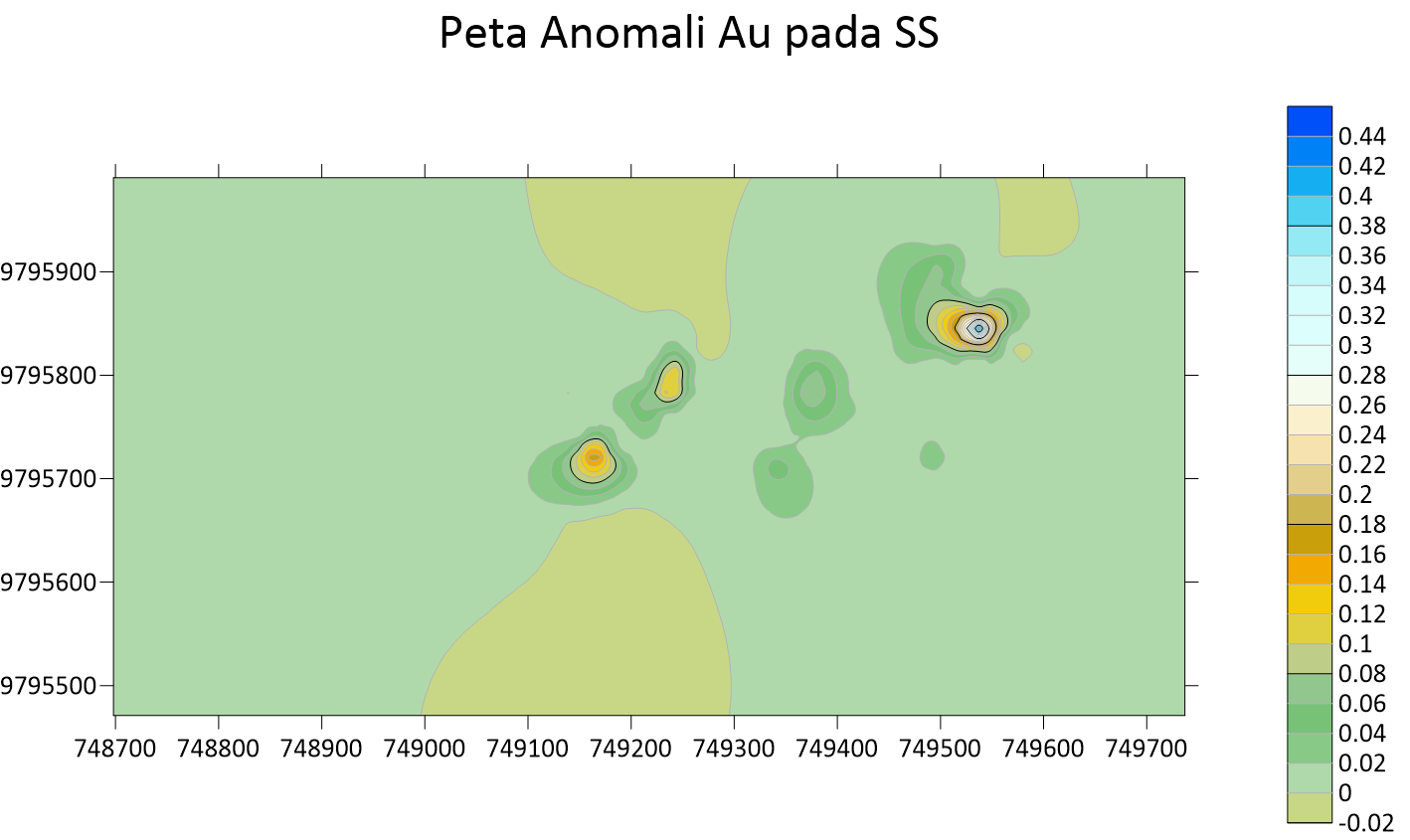 Peta Anomali Au Soil Sampling
 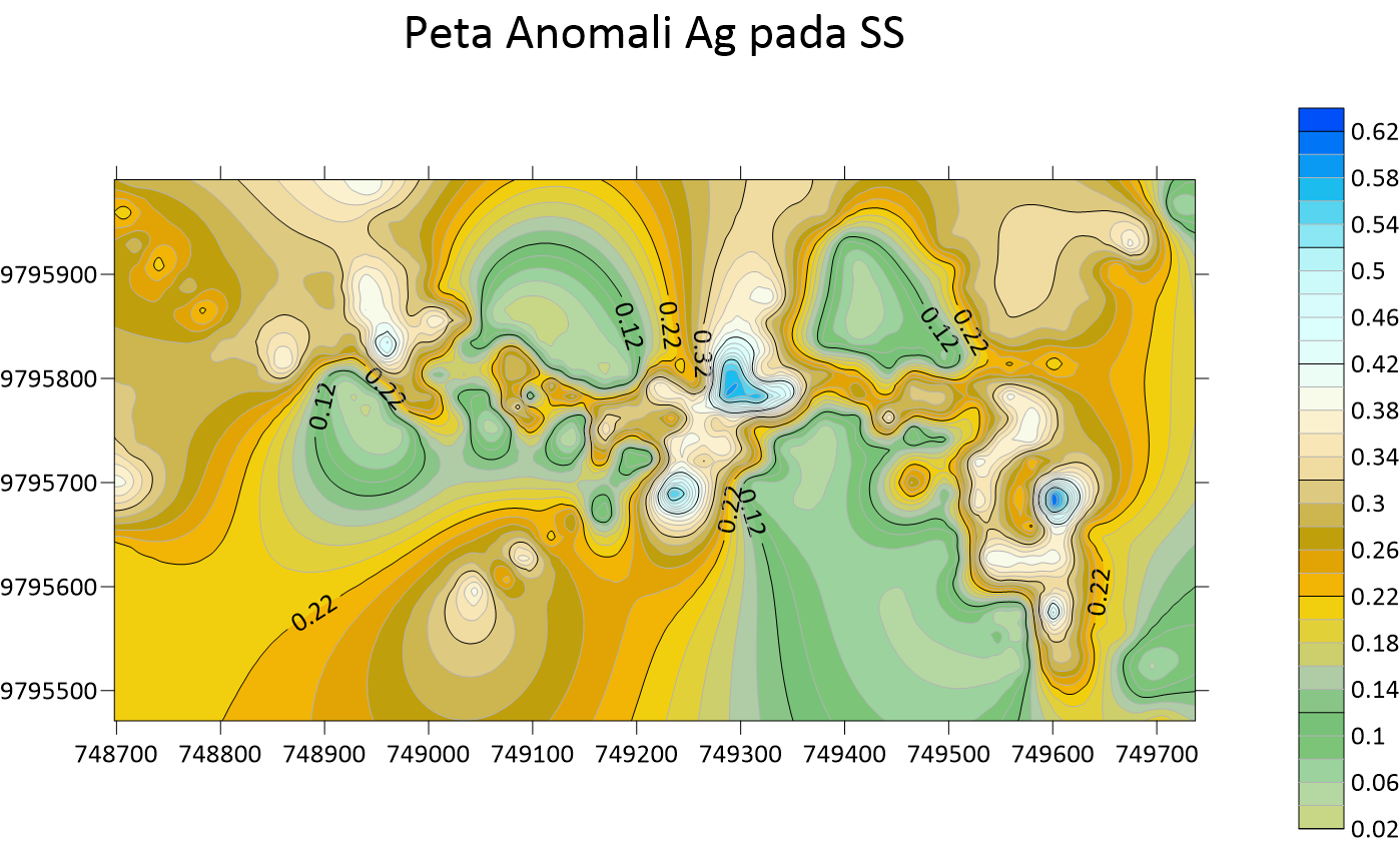 Peta Anomali Ag Soil Sampling
 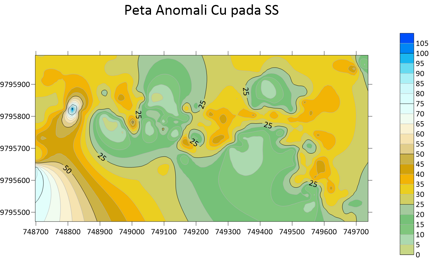 Peta Anomali Cu Soil Sampling
 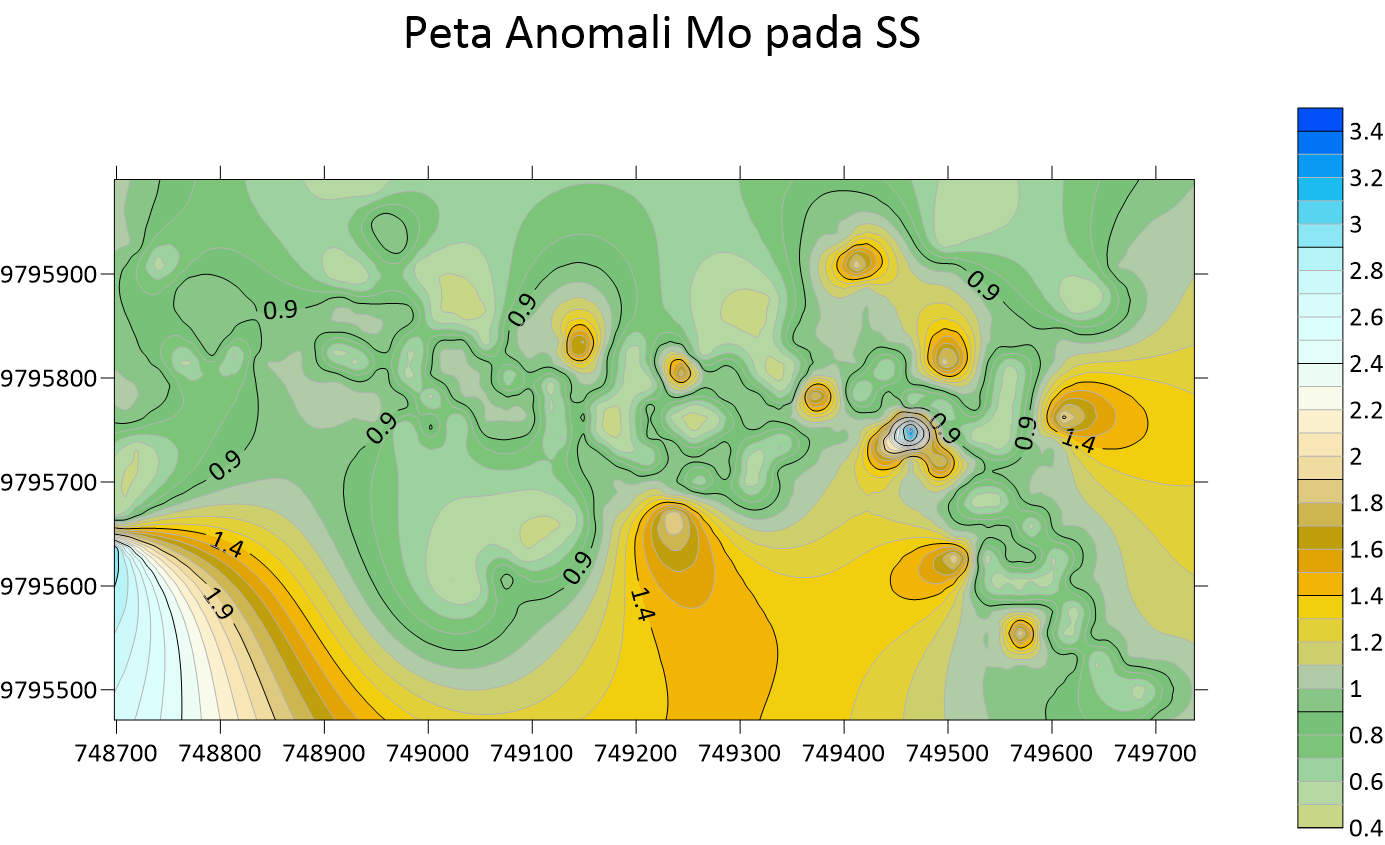 Peta Anomali Mo Soil Sampling
 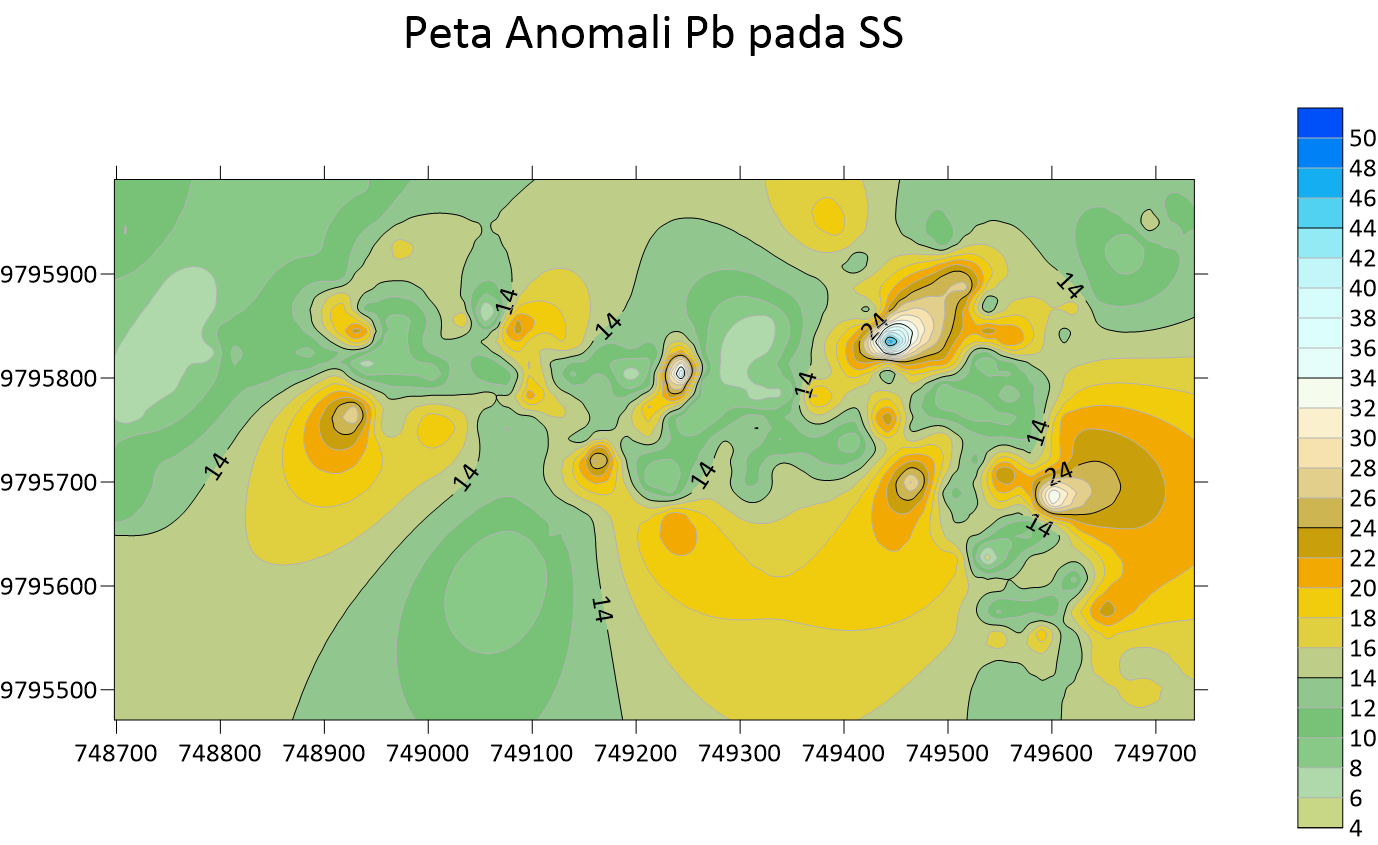 Peta Anomali Pb Soil Sampling
 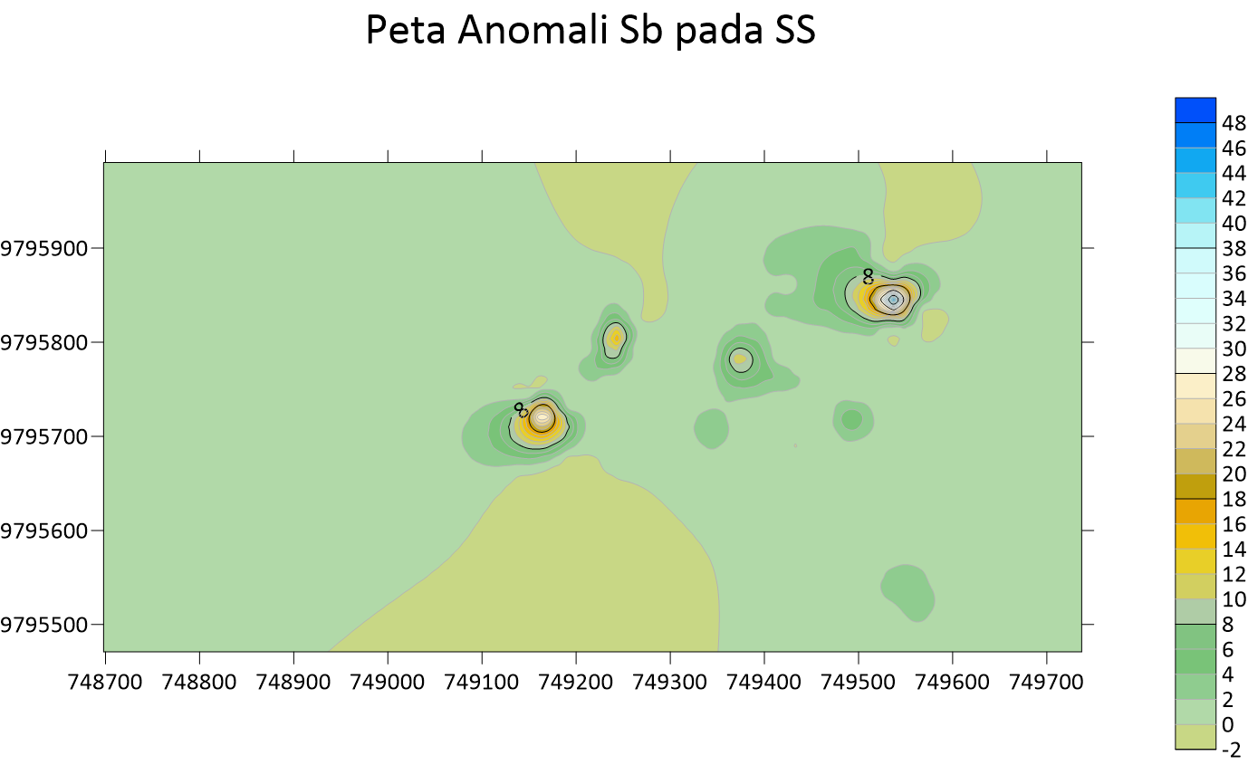 Peta Anomali Sb Soil Sampling
 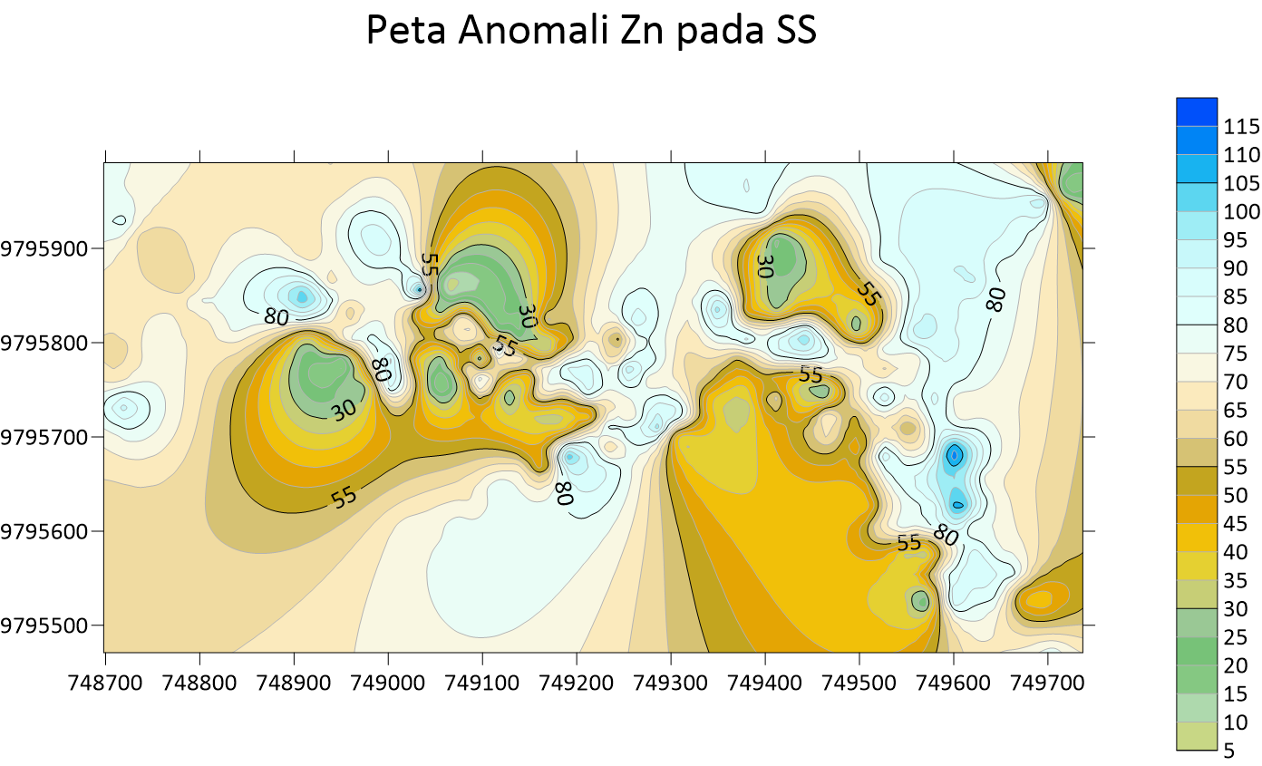 Peta Anomali Zn Soil Sampling